Octave/Matlab Tutorial

Basic Operations

% ======== Math Operators ========= %
5+6
3-2
5*8
3/4
3^5
sqrt(14)

% ======== Logical Opeartors ======= %
4 == 4
2 ~= 4  % Not Equal
1 && 0
1 || 0
xor(1, 0) % XOR

% ======== Other Opeartors ======== %
a = 3
b = "hi"
c = pi  % pi = 3.1416
disp(a)
disp(sprintf('2 decials: %0.2f', a))

% ======== Matrix & Vectors ======= %
M = [1 2 3; 4 5 6; 7 8 9]
V = [1; 2; 3]
A = 1:6 % 1 to 6
B = 1:0.5:3 % Starts from 0 and reaches till 3 with increment of 0.5
C = ones(2, 3) % 2x3 matrix of all 1s
D = 2*ones(2, 3)
E = zeros(1, 3)
W = rand(3, 3) % 3x3 matrix of random numbers --- Normal Distribution
Y = randn(1, 3) % 1 x 3 matrix with numbers follwing mean=0 standard deviation=1 --- Gaussian Distribution
I = eye(4) % 4x4 identity matrix

% ============= Plots ============= %
W = -6 + sqrt(10)*randn(1, 10000)
hist(W) % plots histogram
hist(W, 50) % histogram with 50 bins

% ============= Others ============ %
help(eye)
help(hist)
help(help)
pwd  % present directory
cd % change directory
ls % listy files
who % variables in current scope
whos % with details
clear % clears all variables in scope
a=1, b=2, c=3 % Comma chaning of commands - Mutiple commands one after other

Moving Data Around

M = [1, 2; 3, 4; 5, 6]
size(M) % size of matrix : 3 2
size(M, 1) % Number of rows : 3
size(M, 2) % Number of columns : 2
length(M) % Longest Dimension : 3 -- Often used for vectors
M(3, 2) % Value at 3rd row 2nd column
M(3, :) % Complete 3rd row
M(:, 2) % Complete 2nd column
M([1, 3], :) % Complete 1st and 3rd row
M(:) % Put all elements into a single vector
B = [11, 12; 13, 14; 15, 16]
C = [M, B] % Put B beside matrix M : 3 x 4
D = [M; B] % Put B below matrix M : 6 x 2

% ============ File Handling =========== %
load filename % Loads file data to a variable filename
save test.mat v % Saves variable v in file test.mat
save test.text -ascii % Saves in human readable form

Computing on Data

A = [1, 2; 3, 4; 5, 6]
B = [1; 2]
A*B % No. of columns in 1st matrix should match no. of row in 2nd matrix

C = [11, 12; 13, 14; 15, 16]
A.*C % Element wise multiplication
A.^2 % Element wise squaring of A
log(A) % Element wise logarithm
exp(A) % Element wise exponentian with base e
abs(A) % Element wise mod
-M % Negative of matrix or -1*M
A + 1 % Increment every element by 1
A < 3 % Element wise comparison

% ======= Other Operations ======== %
A' % Transpose of matrix
pinv(A) % Inverse of matrix
magic(5) % 5x5 matrix with property sum of every row, column, diagonal is same
[r, c] = find(A >= 4) % row and col for all the numbers greater or equal to 4
sum(A) % Sum of columns
sum(A, 2) % Sum of rows
prod(A) % Product of columns
prod(A, 2) % Product of rows
floor(A)
ceil(A)
max(A, [], 1) % column wise max
max(A, [], 2) % row wise max

Plotting the Data

t=[0:0.01:0.98]
y1 = sin(2*pi*4*t)
plot(t, y1) % Plots sin graph with t as x-axis and y1 as y-axis
y2 = cos(2*pi*4*t)
plot(t, y2)
plot(t, y1)
hold on % Holds on the previous graph to put another graph on top of it.
plot(t, y2, 'r') % Puts this on top of previous with red color
xlabel('time') % Labels x-axis as time
ylabel('value') % Labels y-axis as value
legend('sin', 'cos') % Marks the color associated to legend on graph
title('muyPlot') % Gives title to graph
print -dpng 'myPlot.png' % Saves the graph as PNG file
help(plot) % To know about plot function
close % Closes the figure to go away

% ========= Figure Commands ========== %
figure(1): plot(t, y1)
figure(2): plot(t, y2)
subplot(1, 2, 1) % Divides plot as 1x2 grid, access first element
plot(t, y1)
subplot(1, 2, 2)
plot(t, y2)
axis([0.5 1 -1 1]) % Changes the scale of the axis
clf % Clears the figure

% ========= Other Commands ========== %
A = magic(5)
imagesc(A) % Draws image with color map as 5x5 matrix
imagesc(A), colorbar % Image with colorbar representing values of color
imagesc(A), colorbar, colormap gray % Changes color and map to gray color bar
imagesc(magic(15)), colorbar, colormap gray % Bigger graph

For, While, If and Functions

% for loop
for i=1:10,
  v(i) = 2^i;
end;

% while loop
i = 1;
while i <=5,
  v(i) = i^2;
  i = i + 1;
end

% if, elseif, else
for i=1:5,
    if(i==1),
        disp('The value is 1');
    elseif i==2,
        disp('The value is 2');
    else
        disp('The value is neither 1 nor 2');
    end;
end;

% if and break statement
while true,
	v(i) = i^2;
	i = i+1;
	if(i==6),
		break;
	end;
end;

% ========== Writing Function ========== %
% Step-1: Create a file called squareNumber.m

% Step-2: Function prototype in file
function [outputArg1,outputArg2] = squareNumber(inputArg1,inputArg2)
	% SQUARENUMBER Summary of this function goes here
  % Detailed explanation goes here
  outputArg1 = inputArg1;
  outputArg2 = inputArg2;
end

% Step-3: Write Actual Function in file and save
function y = squareNumber(x)
    y = x^2;
end

% Call fucntion in terminal
squareNumber(5)
% => 25

% Another Example
[a, b] = squareAndCubeOfNumber(15)

Example-Problem:

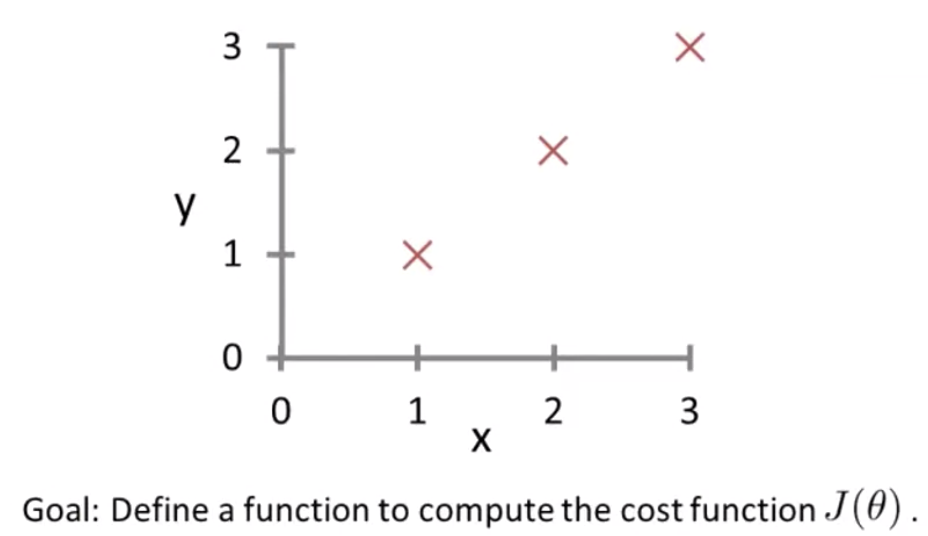
% Function in file costFunctionJ.m
function J = costFunctionJ(X, y, theta)
	% X is "Design Matrix" containing training examples
	% y is class labels
	m = size(X, 1); % No. of training examples = size of rows of Design matrix
	predictions = X*theta; % Predictions of hypothesis on all m examples : predicted_y = X.θ
	sqrErrors = (predictions-y).^2;  % (predicted_val-actual_val)^2 for every element
	J = 1/(2*m)*sum(sqrErrors);
	

% Working of Function
X = [1, 1; 1, 2; 1, 3]
y = [1; 2; 3]
theta = [0; 1] % Fit line as : y = x
costFunctionJ(X, y, theta)
% => 0 : Output Value (All correct predictions with the fit line)

theta = [0; 0] % Change the fit line as y = 0
costFunctionJ(X, y, theta)
% => 2.33 : (1^2 + 2^2 +  3^2)/(2*3) = 2.33  - All wrong predictios with fit line

Vectorization

Whatever programming languages we use have differenrt numerical linear algebra libraries.
They’re usually very well written, highly optimized, often sort of developed by people that are specialized in numerical computing.
When we are implementing machine learning algorithms, we need to take advantage of these linear algebra libraries.