Linear Regression with multiple variables
Multivariate Linear Regression
Linear regression with multiple variables is also known as “multivariate linear regression”.
Multiple Features
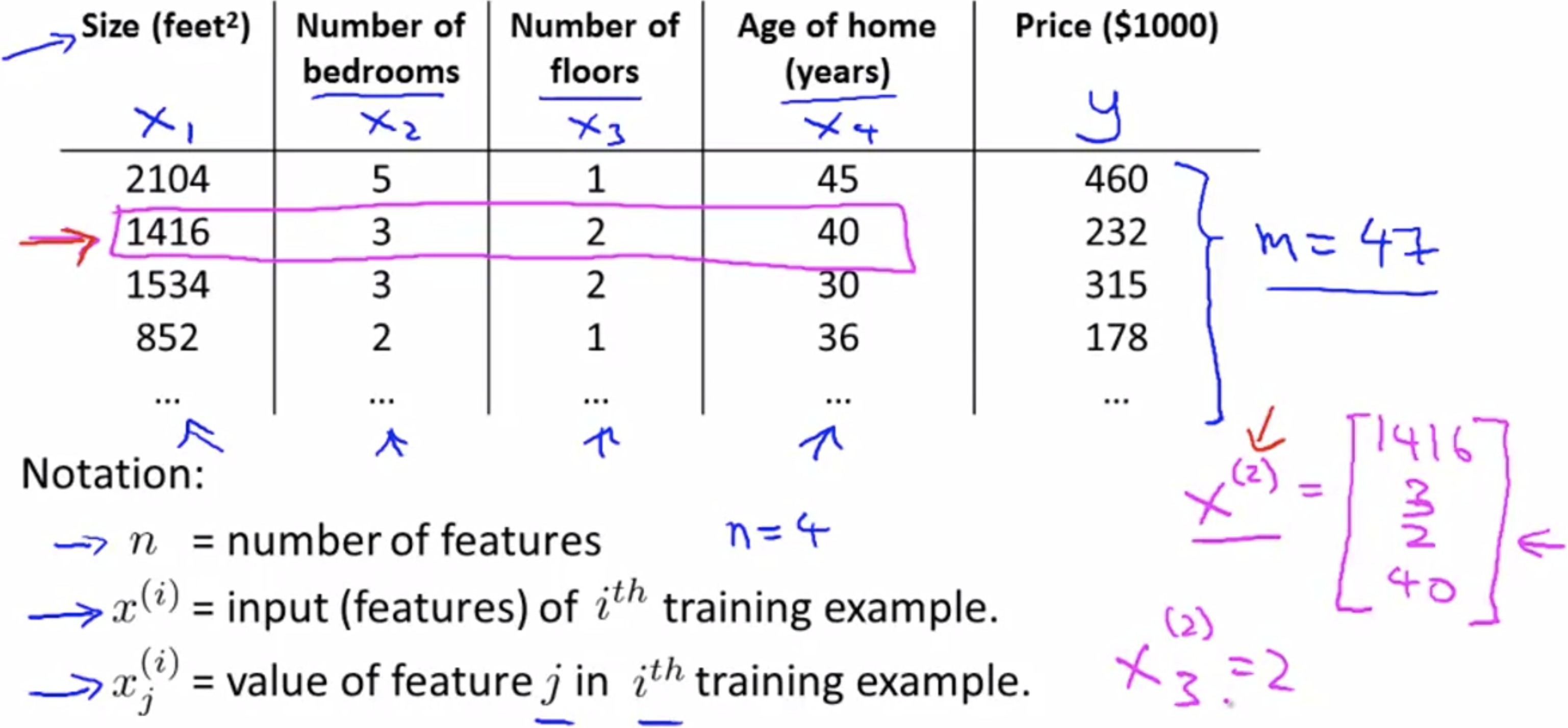
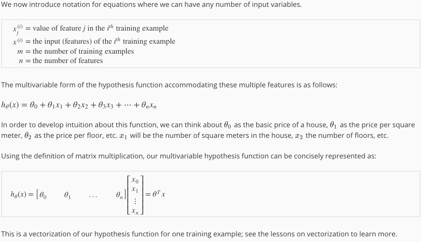
Hypothesis:
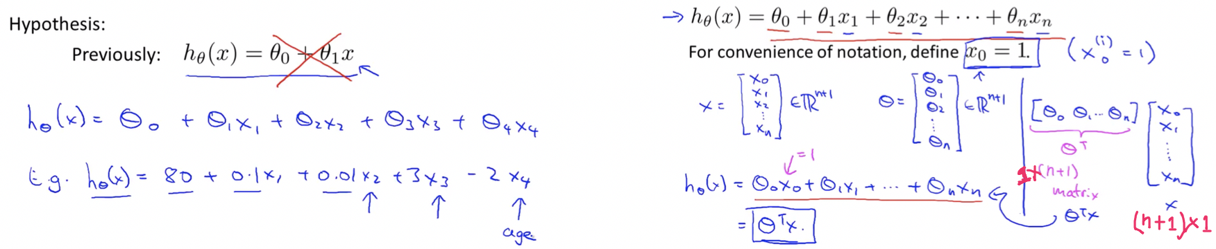
Concepts:
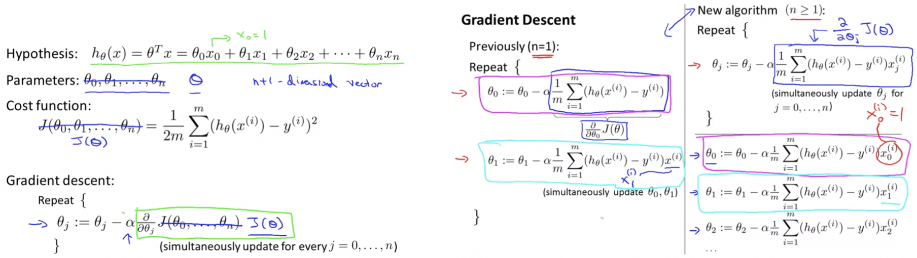
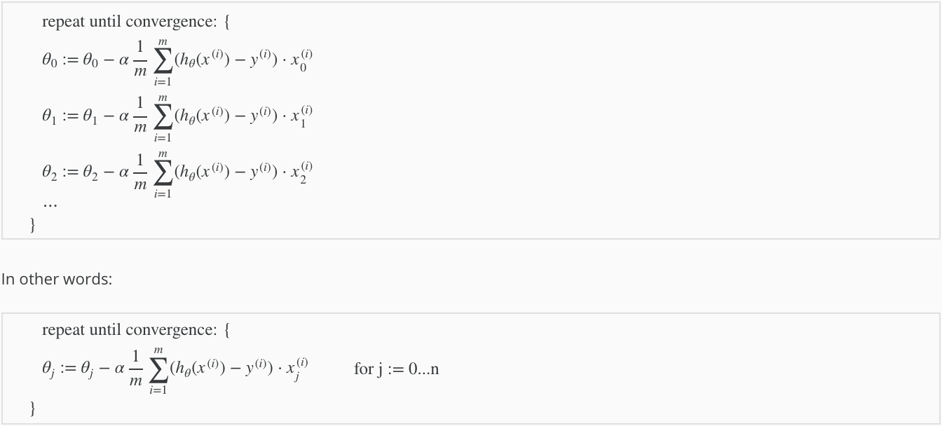
Gradient descent for multiple variables
The gradient descent equation itself is generally the same form; we just have to repeat it for our ‘n’ features:
Concepts:
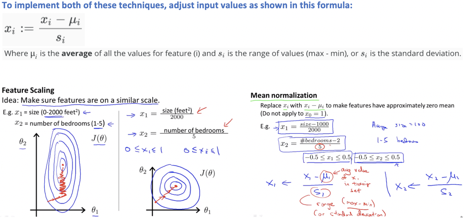
Feature Scaling:
We can speed up gradient descent by having each of our input values in roughly the same range.
This is because θ will descend quickly on small ranges and slowly on large ranges, and so will oscillate inefficiently down to the optimum when the variables are very uneven.
The way to prevent this is to modify the ranges of our input variables so that they are all roughly the same.
Ideally: −1 ≤ x(i) ≤ 1 or 0.5 ≤ x(i) ≤ 0.5
Two techniques to help with this are:
- Feature Scaling: Involves dividing the input values by the range (i.e. the maximum value minus the minimum value) of the input variable, resulting in a new range of just 1.
- Mean Normalization: Mean normalization involves subtracting the average value for an input variable from the values for that input variable resulting in a new average value for the input variable of just zero.
Learning Rate:
Job of gradient descent is to find the value of θ that hopefully minimizes the cost function J(θ).
Debugging gradient descent:
- Make a plot with number of iterations on the x-axis.
- Now plot the cost function, J(θ) over the number of iterations of gradient descent.
- If J(θ) ever increases, then probably need to decrease α.
Automatic convergence test:
- Declare convergence - if J(θ) decreases by less than ε in one iteration, where ε is some small value such as 10−3.
- However in practice it’s difficult to choose this threshold value.
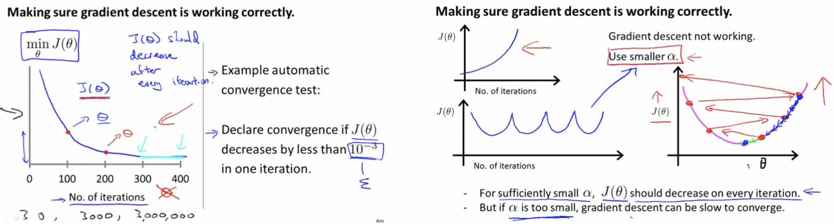
Summary:
- If α is too small: slow convergence.
- If α is too large: may not decrease on every iteration and thus may not converge.
To choose α try: . . . . . . , 0.001, 0.003, 0.01, 0.03, 0.1, 0.3, 1, 3, 10, 30, 100, . . . . . . . . .
Features and Polynomial Regression
- Sometimes by defining new features we might actually get a better model than that of given features.
- Example: In case of house price prediction instead of using 2 given features length and breadth, we can define new feature area.
- Closely related to the idea of choosing our own features is the idea called polynomial regression.
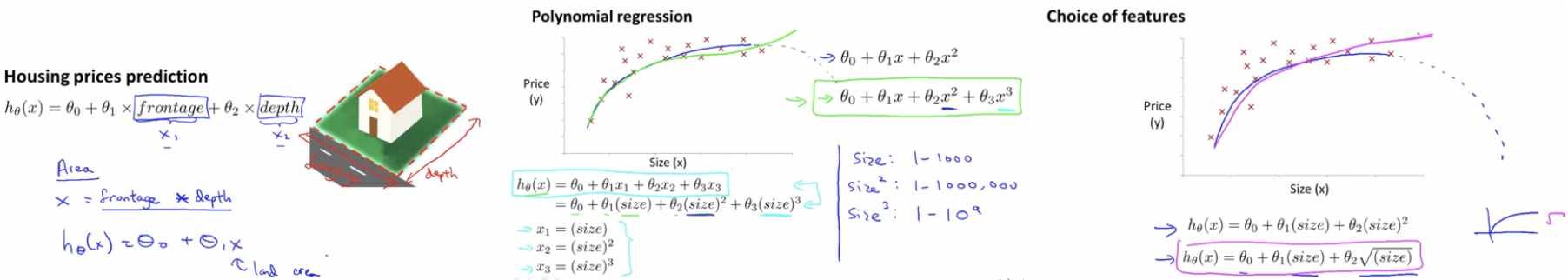
Note:
If you choose our features in the way like squares and cubes then feature scaling becomes very important.
Computing Parameters Analytically
Gradient descent gives one way of minimizing cost function J.
Let’s discuss a second way of doing so, this time performing the minimization explicitly and without resorting to an iterative algorithm.
Normal Equation Method
- We minimize J(θ) by explicitly taking its derivatives with respect to the θj ’s, and setting them to zero.
- This allows us to find the optimum theta without iteration.
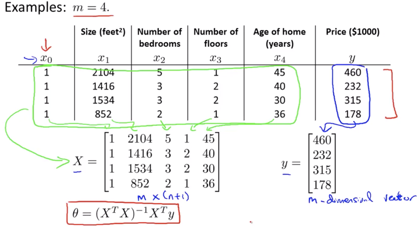
Normal Equation Formula: θ = (XTX)-1XTy
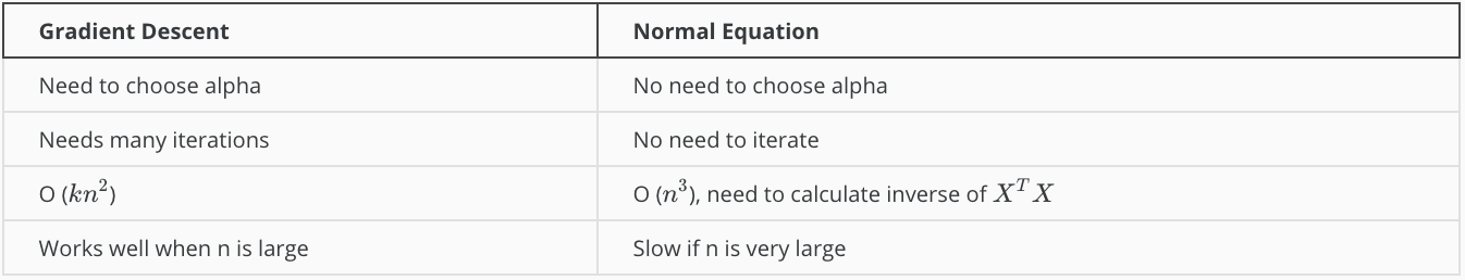
Gradient Descent Vs. Normal Equation:
Notes:
- There is no need to do feature scaling with the normal equation.
- With the normal equation, computing the inversion has complexity O(n3), so if we have a very large number of features, the normal equation will be slow.
- In practice, when n exceeds 10,000 it might be a good time to go from a normal solution to an iterative process.
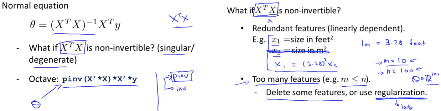
Normal Equation: Non-invertibility
- Not all matrices are invertible, non-invertible matrices are also called singular/degenerate.
- When implementing the normal equation in octave we want to use the
'pinv'function rather than'inv'. - The
'pinv'function gives a value of θ even if XTX is not invertible.
If XTX* is noninvertible, the common causes might be having :
- Redundant features, where two features are very closely related (i.e. they are linearly dependent).
- Too many features (e.g. m ≤ n). In this case, delete some features or use “regularization”.
Next: Octave/Matlab Tutorial →